Algorithms in Kotlin, Big-O-Notation, Part 1/7
![]()

- Introduction
- Algorithmic performance and asymptotic behavior
- O(1)
- O(n)
- O(n^2)
- O(2^n)
- O(log n)
- O(n * log n)
- Resources
Introduction #
This tutorial is part of a collection tutorials on basic data structures and algorithms that are created using Kotlin. This project is useful if you are trying to get more fluency in Kotlin or need a refresher to do interview prep for software engineering roles.
How to run this project #
You can get the code for this and all the other tutorials in this collection from this github repo. Here’s a screen capture of project in this repo in action.
Once you’ve cloned the repo, type ./gradlew run in order to build and run this project from the
command line.
Importing this project into JetBrains IntelliJ IDEA #
- This project was created using JetBrains Idea as a Gradle and Kotlin project (more info). - When you import this project into Idea as a Gradle project, make sure not to check “Offline work” (which if checked, won’t allow the gradle dependencies to be downloaded). - As of Jun 24 2018, Java 10 doesn’t work w/ this gradle distribution (v4.4.x), so you can use Java 9 or 8, or upgrade to a newer version of gradle (4.8+).
Algorithmic performance and asymptotic behavior #
To meaningfully compare algorithmic performance, we can use big O notation – sometimes referred to as “order of growth.” In short, it compares the asymptotic behavior of algorithms; that is, how does their performance scale as a function of the input size?
O(1) #
An algorithm that will always execute in the same time (or space) regardless of the size of the input data set.
fun isFirstElementNull(list: List<String?>) = list[0]==null
O(n) #
An algorithm whose performance will grow linearly and in direct proportion to the size of the input data set. Big O favors the worst-case performance scenario.
fun containsValue(list: List<String>, value: String): Boolean {
    list.forEach { it ->
        if (it == value) return true
    }
    return false
}
The example above demonstrates how Big O favours the worst-case performance scenario; a matching string could be found during any iteration of the for loop and the function would return early, but Big O notation will always assume the upper limit where the algorithm will perform the maximum number of iterations.
Counting sort #
Counting sort is an efficient algorithm for sorting an array of elements that each have a non-negative integer key, for example, an array, sometimes called a list, of positive integers could have keys that are just the value of the integer as the key, or a list of words could have keys assigned to them by some scheme mapping the alphabet to integers (to sort in alphabetical order, for instance). Unlike other sorting algorithms, such as merge sort, counting sort is an integer sorting algorithm, not a comparison based algorithm.
- Any comparison based sorting algorithm requires O(n * log n) comparisons (more on this below).
- Counting sort has a running time of O(n) when the length of the input list is not much smaller than the largest key value, k, in the list.
- The space-time complexity of counting sort really amounts to a combination of both the number of elements to be sorted, n, and the range between the largest and smallest element, or k. The true Big O notation of counting sort is O(n + k). However, counting sort is generally only ever used if k isn’t larger than n; in other words, if the range of input values isn’t greater than the number of values to be sorted. In that scenario, the complexity of counting sort is much closer to O(n), making it a linear sorting algorithm.
Counting sort can be used as a subroutine for other, more powerful, sorting algorithms such as radix sort.
/**
 * Create temp array called `countingArray` to count the # occurrences of each
 * value in the list.
 * - The index of the countingArray maps to values of items in the list.
 * - countingArray[index] maps to # occurrences of that value.
 */
fun counting_sort(list: MutableList<Int>) {
    val countingArray = IntArray(if (list.max() == null) 0 else list.max()!! + 1)
    for (item in list) countingArray[item]++

    // Regenerate the list using the countingArray
    var cursor = 0
    for (index in 0 until countingArray.size) {
        val value = index
        val numberOfOccurrences = countingArray[index]
        if (numberOfOccurrences > 0)
            repeat(numberOfOccurrences) {list[cursor++] = value}
    }
}
Counting sort has a O(k+n) running time.
- The first loop goes through A, which has n elements. This step has a O(n) running time. k is the highest value in this list + 1.
- The second loop iterates over k, so this step has a running time of O(k).
- The third loop iterates through A, and this has a running time of O(n). Therefore, the counting sort algorithm has a running time of O(k+n).
Counting sort is efficient if the range of input data, k, is not significantly greater than the number of objects to be sorted, n.
Counting sort is a stable sort with a space complexity of O(k+n).
O(n^2) #
O(n^2) (or quadratic) represents an algorithm whose performance is directly proportional to the square of the size of the input data set. This is common with algorithms that involve nested iterations over the data set such as the example below.
Detect duplicates #
fun containsDuplicates(list: List<String>) : Boolean {
    with(list) {
        for (cursor1 in 0 until size) {
            for (cursor2 in 0 until size) {
                if (cursor1 != cursor2) {
                    if (get(cursor1) == get(cursor2)) return true
                }
            }
        }
    }
    return false
}
Deeper nested iterations will result in O(n^3), O(n^4) etc.
Bubble sort #
Here’s an example of Bubble sort which is also O(n^2). For a list size of 4, this creates 6
comparisons and up to 6 swaps (which is (4-1)!). More info on
factorial functions.
In the first pass of the x loop, this simplistic algorithm bubbles the highest / lowest item to
the top of the list. Then it does x+1 .. size-1 loops (for each subsequent pass of the x loop)
to bubble the highest / lowest remaining item to the rest of the array indices.
/** O(n^2) */
fun bubble_sort(list: MutableList<String>) {
    val size = list.size

    for (x in 0 until size) {
        for (y in x + 1 until size) {
            println("\tx=$x, y=$y")
            if (list[y] < list[x]) {
                list.swap(y, x)
            }
        }
    }
}

fun <T> MutableList<T>.swap(index1: Int, index2: Int) {
    val tmp = this[index1] // 'this' is a reference to the list.
    this[index1] = this[index2]
    this[index2] = tmp
}
O(2^n) #
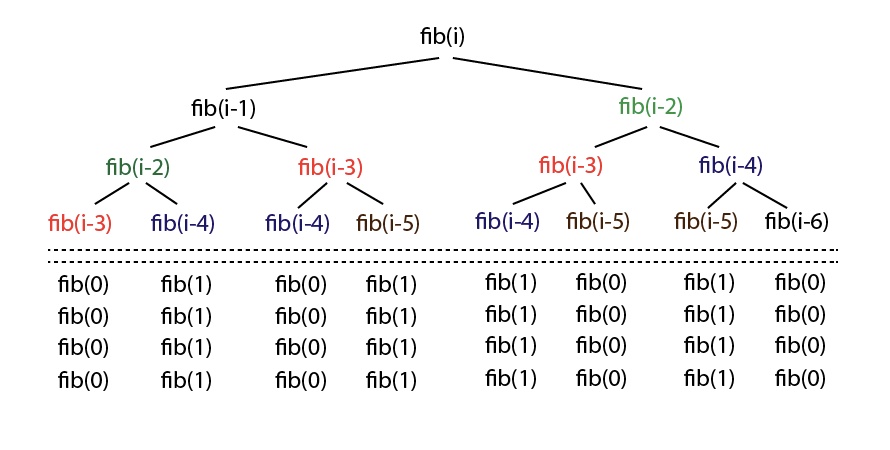
O(2^n) denotes an algorithm whose growth doubles with each addition to the input data set. The growth curve of an O(2^n) function is exponential - starting off very shallow, then rising meteorically or asymptotically. Exponentiation is the inverse mathematical function of logarithm. Here’s an example of an O(2^n) function is the recursive calculation of Fibonacci numbers.
fun fib(number: Int): Int =
    if (number <= 1) number
    else fib(number - 1) + fib(number - 2)
Here’s a visual representation of the call stack, showing how the program just recomputes the values for the same things repeatedly.
O(log n) #
Binary Search #
Binary search is a technique used to search sorted data sets. It works by selecting the middle element of the data set, essentially the median, and compares it against a target value.
- If the values match it will return success.
- If the target value is higher than the value of the probe element it will take the upper half of the data set and perform the same operation against it.
- Likewise, if the target value is lower than the value of the probe element it will perform the operation against the lower half.
It will continue to halve the data set with each iteration until the value has been found or until it can no longer split the data set.
This type of algorithm is described as O(log n).
- The iterative halving of data sets described in the binary search example produces a growth curve that peaks at the beginning and slowly flattens out as the size of the data sets increase.
- Using a binary search, i.e. splitting the remaining part of an array into equal parts iteratively, will allow us to zero in on the element.
- At most, it will take log-base-2(n) splits to find the element, so this algorithm is in O(log n) time.
For example if an input data set containing 10 items takes one second to complete, then
- a data set containing 100 items takes two seconds,
- and a data set containing 1000 items will take three seconds.
Doubling the size of the input data set has little effect on its growth as after a single iteration of the algorithm the data set will be halved and therefore on a par with an input data set half the size. This makes algorithms like binary search extremely efficient when dealing with large data sets.
For a more in-depth explanation take a look at their respective Wikipedia entries: Big O Notation, Logarithms.
fun binarySearch(item: String, list: List<String>): Boolean {
    // Exit conditions (base cases)
    if (list.isEmpty()) {
        return false
    }

    // Setup probe
    val probeIndex = list.size / 2
    val probeItem = list[probeIndex]

    // Does the probe match? If not, split and recurse
    when {
        item == probeItem -> return true
        item < probeItem -> return binarySearch(item,
                                                list.subList(0, probeIndex))
        else -> return binarySearch(item,
                                    list.subList(probeIndex + 1, size))
    }
}
O(n * log n) #
Merge Sort #
Merge sort is an algorithm that is n * log n in runtime complexity. It’s a divide and conquer algorithm that splits a given list in half recursively, until each list only has 1 element in it. Then it merges these lists back into one big list by sorting each one of these smaller lists and merging them back up into larger and larger lists.
- The number of stages of the divide and conquer phase where the main list is recursively split and then merged back, is O(log n).
- For each O(log n) stage, about O(n) comparisons need to be made (after the divide phase) to compare and merge these smaller lists back into larger and larger lists.
- So it ends up being O(n * log n).
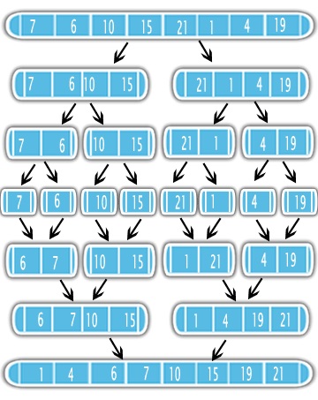
The following animation visually depicts how this divide and conquer algorithm works on data. It leverages the fact that it’s inexpensive to merge two (already) sorted lists together. So, this algorithm recursively splits the main lists into smaller lists, until each the smallest list just has a single element in it. Then proceeds to merge these lists of 1 element each back into larger lists. Each of these larger lists are sorted as they’re assembled, so this takes advantage of merging two smaller sorted lists into a larger list.
Here’s the runtime of the algorithm visualized on a sample data set.
/**
 * O(n * log(n))
 *
 * This function doesn't actually do any sorting (actually done in [merge]).
 * - O(log(n)) -> recursively splitting the given list into smaller lists.
 * - O(n) -> merging two pre-sorted lists quickly (the [merge] function).
 *
 * [Graphic depicting merge sort in action](http://bit.ly/2u1HuNp).
 *
 * We can also describe the steps of the algorithm a little differently:
 *
 * 1) Split the n elements of the list into n separate lists, each of size one.
 * 2) Pair adjacent lists and merge them, resulting in about half as many lists
 *    each about twice the size.
 * 3) Repeat step 2 until you have one list of size n.
 *
 * After the last recursive calls, we are operating on arrays of size 1, which
 * cannot be split any further and are trivially sorted themselves, thus giving
 * us our base case.
 *
 * Please note that [quick_sort] on average runs 2-3 times faster merge sort.
 */
fun merge_sort(list: MutableList<String>): MutableList<String> {
    // Can't split lists anymore, so stop recursion
    val length = list.size
    if (length <= 1) return list

    // Split the list into two and recurse (divide)
    val middleIndex = length / 2
    val leftList = merge_sort(list.subList(0, middleIndex))
    val rightList = merge_sort(list.subList(middleIndex, length))

    // Merge the left and right lists (conquer)
    return merge(leftList, rightList)
}

/**
 * In this step, the actual sorting of 2 already sorted lists occurs.
 *
 * The merge sort algorithm takes advantage of the fact that two sorted
 * lists can be merged into one sorted list very quickly.
 */
fun merge(leftList: MutableList<String>, rightList: MutableList<String>):
        MutableList<String> {
    val result = mutableListOf<String>()
    var leftIndex = 0
    var rightIndex = 0

    while (leftIndex < leftList.size && rightIndex < rightList.size) {
        val lhs = leftList[leftIndex]
        val rhs = rightList[rightIndex]
        if (lhs < rhs) {
            result.add(lhs)
            leftIndex++
        } else {
            result.add(rhs)
            rightIndex++
        }
    }

    // Copy remaining elements of leftList (if any) into the result
    while (leftIndex < leftList.size) {
        result.add(leftList[leftIndex])
        leftIndex++
    }

    // Copy remaining elements of rightList (if any) into the result
    while (rightIndex < rightList.size) {
        result.add(rightList[rightIndex])
        rightIndex++
    }

    return result
}
Quick Sort #
Quick sort is another divide and conquer algorithm with better performance than merge sort. The main difference between quick sort and merge sort is that for quick sort, all the “heavy” lifting is done while the list is being split in two, whereas with merge sort, we simply split the list in two and worry about sorting it later.
Unlike merge sort, this algorithm performs a one pass mini sort on a portion of the list, before splitting it. This is different than merge sort, where the list is split in half recursively and the sorting occurs during the merge phase.
In quick sort, the list is partitioned by picking an arbitrary value (a pivot value), which is typically the last element of the list itself. This partition function then puts all the values that are smaller than it to the left of the list, and the ones higher than it to the right of the list, then is moved into the correct position in the list (not necessarily the middle). Then recursively, the list is split to the left and right of this pivot, until there’s nothing left to split.
Divide - When you divide the list into two, you pick a pivot point (typically the last element of the array) and then all the elements smaller than it get moved to the left of it, and all of those larger than it get moved to the right of it, so the pivot point is effectively moved to its ultimate sorted position.
Conquer - All elements to the left are fed recursively back into the algorithm, as are elements to the right until the entire list is sorted.
This algorithm has really low memory footprint, since the items are swapped in place in the same array, unlike merge sort, which can take up more memory.
If the pivot point is in the middle of all the values in the set each time, the runtime approaches O(n * log n). However, if it is close to one of the minimum or maximum each time it approaches its worst case O(n^2), although this is rare.
It’s true that the worst case runtime for quick sort is higher (in the case of pre-sorted data, or data that’s inverse sorted), but this case is very rare, and in fact, quick sort outperforms merge sort (on average) for reasonably randomized data. This is due to its cache performance and the simplicity of the operations involved in the innermost loop. Overall, these advantages make quick sort 2-3 times faster (on average) than merge sort for large data sets.
/**
 * O(n * log(n))
 *
 * Quick sort on average runs 2-3 times faster than [merge_sort].
 *
 * If the data is mostly pre-sorted, then the runtime performance will
 * be worse than expected, and will approach O(n^2). Ironically, the
 * pre-sorted data takes longer to sort than the “random” data. The
 * reason is because the pivot point will always be picked
 * sub-optimally, with a “lopsided” partitioning of the data.
 * When we pick this "lopsided" pivot, we are only reducing the problem
 * size by one element. If the pivot were ideal, we would be reducing
 * the problem size by half, since roughly half of the elements would
 * be to the left of the pivot and the other half to the right.
 */
fun quick_sort(list: MutableList<Int>,
               startIndex: Int = 0,
               endIndex: Int = list.size - 1) {
    if (startIndex < endIndex) {
        val pivotIndex = partition(list, startIndex, endIndex)
        quick_sort(list, startIndex, pivotIndex - 1) // Before pivot index
        quick_sort(list, pivotIndex + 1, endIndex) // After pivot index
    }
}

/**
 * This function takes last element as pivot, places the pivot
 * element at its correct (final) position in (fully) sorted list,
 * and places all smaller (smaller than pivot) to left of pivot
 * and all greater elements to right of pivot.
 *
 * Ideally this pivot element would represent the median of the
 * sublist. But in this implementation we are choosing the end
 * of the sublist (the element at endIndex).
 */
fun partition(list: MutableList<Int>,
              startIndex: Int = 0,
              endIndex: Int = list.size - 1): Int {
    // Element to be placed at the correct position in the list
    val pivotValue = list[endIndex]

    // Index of element smaller than pivotValue
    var smallerElementIndex = startIndex

    // Make a single pass through the list (not including endIndex)
    for (index in startIndex until endIndex) {
        // If current element is smaller than equal to pivotValue then swap it w/
        // the element at smallerElementIndex
        val valueAtIndex = list[index]
        if (valueAtIndex < pivotValue) {
            list.swap(smallerElementIndex, index)
            smallerElementIndex++
        }
    }

    // Finally move the pivotValue into the right place on the list
    list.swap(smallerElementIndex, endIndex)

    // Return the index just after where the pivot value ended up
    return smallerElementIndex
}

fun MutableList<Int>.swap(index1: Int, index2: Int) {
    val tmp = this[index1] // 'this' corresponds to the list
    this[index1] = this[index2]
    this[index2] = tmp
}
Resources #
CS Fundamentals #
- Brilliant.org CS Foundations
- Radix sort
- Hash tables
- Hash functions
- Counting sort
- Radix and Counting sort MIT
Data Structures #
Math #
- Khan Academy Recursive functions
- Logarithmic calculator
- Logarithm wikipedia
- Fibonacci number algorithm optimizations
- Modulo function
Big-O Notation #
- Asymptotic complexity / Big O Notation
- Big O notation overview
- Big O cheat sheet for data structures and algorithms
Kotlin #
- Using JetBrains Idea to create Kotlin and gradle projects, such as this one
- How to run Kotlin class in Gradle task
- Kotlin
untilvs.. - CharArray and String
Markdown utilities #
👀 Watch Rust 🦀 live coding videos on our YouTube Channel.
📦 Install our useful Rust command line apps usingcargo install r3bl-cmdr(they are from the r3bl-open-core project):
- 🐱
giti: run interactive git commands with confidence in your terminal- 🦜
edi: edit Markdown with style in your terminalgiti in action
edi in action